Overview
In this vignette, we provide a detailed tutorial of the key
functionalities of the RaCE.NMA R package. The package has
functions to complete three primary tasks in the analysis pipeline when
utilizing the RaCE-NMA methodology:
- Model estimation
- Model assessment
- Inference and summary statistics
After loading the necessary packages to run our analyses, we demonstrate each of the primary tasks in the analysis pipeline on two datasets: A toy dataset (as seen in Simulation Study 2 of the paper) and real data (as seen in the Case Study of the paper).
Toy Data
First, we use a “toy” dataset that can be seen in Simulation Study 2
of the paper. The data is included in the RaCE.NMA package
and can be loaded using the following code:
data("toy_data")
head(toy_data)
#>           V1           V2       V3         V4
#> 1 -1.0896915  0.018484918 1.158785 -1.1303757
#> 2 -1.0080252  0.013242028 1.070795 -0.2396980
#> 3 -0.8015526 -0.013878701 1.041765  0.9817528
#> 4 -1.0392695 -0.103966898 1.178223 -2.3110691
#> 5 -0.9121395  0.003580672 1.101283  0.4322652
#> 6 -0.7909181 -0.119992582 1.158964  1.9546516
The data contains rows and 4 columns. Each column represented a treatment, and each row a posterior draw of relative treatment effects for those treatments. We assume these posterior draws are based on a standard NMA model (i.e., no rank-clustering).
To visualize these posterior draws, we create a forest plot (with 95%
CIs) via the aptly-named create_forestplot function:
forestplot_muhat(data = toy_data, level = 0.95,
                  order_by_average = FALSE)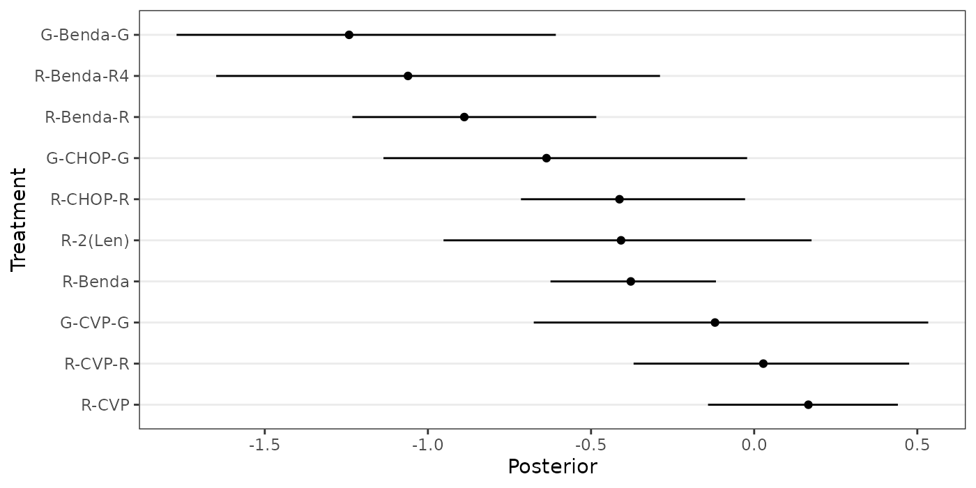
Figure 1: Forest plot of estimated relative treatment effects in a toy example dataset, based on a standard NMA model.
We observe that the first three treatments have narrow and well-separated credible intervals of relative efficacy. The fourth treatment, however, has a very wide interval to indicate high uncertainty in its relative efficacy.
Now we are ready to start the analysis pipeline.
1. Model Estimation
The RaCE.NMA packages contains a primary model-fitting
function, mcmc_RCMVN. The function requires many inputs,
which may be broken down into three categories:
- Previous results from an NMA analysis: The user must provide results on the relative treatment effects from a previous NMA study. Various formats are allowed; see below.
- Model hyperparameters: Parameters which correspond to “priors” in the Bayesian model. Vague priors are available by default.
- MCMC settings: Specifications of an MCMC estimation procedure, including the number of independent chains, length of each chain, thinning and burn-in, etc. By default, the function runs 2 chains, each of length 15000 and removes the first half of iterations as burn-in.
Results of a standard NMA model
If available, we recommend inputting the full posterior of the
relative treatment effect from a previous NMA analysis into the
mcmc_RCMVN function. In this case, the
posterior argument should be provided an
matrix, where the (i,j) entry indicates the relative treatment effect of
treatment
in MCMC draw
.
An example of this functionality is provided below:
mcmc_raceNMA(posterior = toy_data)In the above code, default settings are used for all other inputs. (We recommend against this practice.)
Alternatively, one may provide summary statistics of the model posterior (instead of a full posterior itself). This is useful when applying the RaCE-NMA methodology to the results of a published paper post-hoc, when only summary statistics are available. In this setting, the user must provide two inputs:
-
mu_hat: A vector of length (the number of treatments), where the th entry displays the average relative treatment effect of treatment -
covors: A covariance matrix of relative treatment effects or a vector of length of treatment-specific standard deviations of relative treatment effects.
An example of this functionality is provided below:
mcmc_raceNMA(mu_hat = mu_hat_toy, cov = cov_toy) # example with mu_hat and cov
mcmc_raceNMA(mu_hat = mu_hat_toy, s   = s_toy  ) # example with mu_hat and s
If duplicative inputs are provided, the function will always use those provided the “richest” information. Specifically,
- If
posterioris provided,mu_hat,cov, and/orswill be ignored. - If
covis provided,sis ignored.
Model hyperparameters
Next, we may specify the following hyperparameters:
-
mu0: The prior mean on the rank-clustered relative treatment effects. Defaults tomean(mu_hat), which aims to be vague. -
sigma0: The prior standard deviation on the rank-clustered relative treatment effects. Defaults tosqrt(10*var(mu_hat)), which aims to be vague.
The following code demonstrates how one could specify these hyperparameters directly in the estimation function:
mcmc_raceNMA(
  posterior = toy_data, # results of a standard NMA model
  mu0 = mean(mu_hat_toy), sigma0 = sqrt(10*var(mu_hat_toy)), # model hyperparameters
)
MCMC settings
Last, we may specify parameters that control how the MCMC chains are run:
-
tau: The standard deviation of the Metropolis Hastings proposal distribution. Defaults tomin(|mu_hat_i-mu_hat_j|). -
nu0: How cluster-specific mean parameters are initialized. Defaults toNULL, which randomly samples from the prior distribution. -
iter: The number of times the rank-clustering structure is sampled in each MCMC chain. Defaults to . -
nu_iter: The number of times each cluster-specific mean is sampled per sampling of the rank-clustering structure. Defaults to . In total, there will beiternu_itersamples from the posterior. -
chains: The number of independent MCMC chains. Defaults to 2. -
burn_prop: The proportion of MCMC samples in each chain to be removed as burn-in. Defaults to 0.5. -
thin: A number indicating how often to thin samples. Defaults to 1, indicating no thinning. -
seed: The random seed to run chains. Defaults toNULL, meaning the environment seed is inherited.
The following code demonstrates how one could specify some of these settings directly in the estimation function:
mcmc_results_toy <- mcmc_raceNMA(
  posterior = toy_data, # results of a standard NMA model
  mu0 = mean(mu_hat_toy), sigma0 = sqrt(10*var(mu_hat_toy)), # model hyperparameters
  iter = 10000, nu_iter = 2, # MCMC settings
  chains = 2, burn_prop = 0.5, thin = 1, seed = 1
)
#> [1] "Estimating chain 1 of 2."
#> [1] "Estimating chain 2 of 2."
2. Model Assessment
The package contains three functions to assess if the MCMC chains
have converged and mixed. The first two produce trace plots of
mu and K, the primary model parameters. The
third calculates the
statistic for each mu parameter. We display and interpret
each plot below.
traceplot_mu(mcmc_results_toy)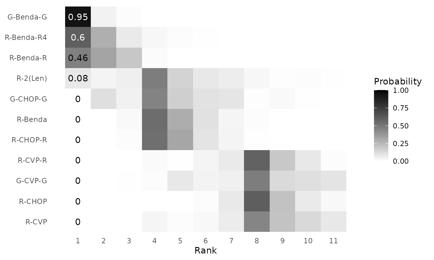
Figure 2: Trace plots of relative treatment effects in a toy example dataset, based on the RaCE-NMA model.
We observe acceptable mixing and convergence in the trace plots for . Ideally, the two chains would like similar to each other, with each exhibiting a “white noise pattern”. This is certainly true for , , and . For , we notice some “jumps” in value across iterations. Based on our toy data, in which treatment 4 has extremely high uncertainty, we expect this type of behavior. Furthermore, since the chains both exhibit similar patterns, we are satisfied.
traceplot_K(mcmc_results_toy)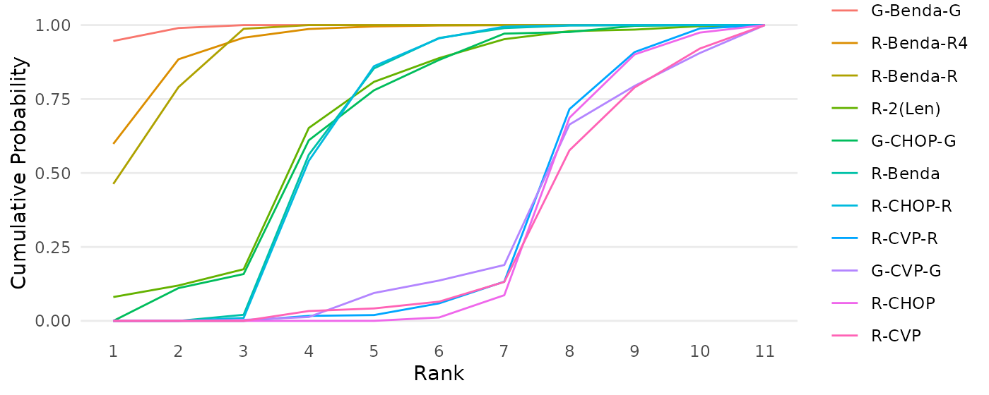
Figure 3: Trace plot of the number of rank-clusters, K, in a toy example dataset, based on the RaCE-NMA model.
We again observe acceptable mixing and convergence in the trace plot for . That is, the two chains are indistinguishable and exhibit a seemingly random pattern between the values and .
calculate_Rhat(mcmc_results_toy, level = 0.9)
#> Potential scale reduction factors:
#>
#>     Point est. Upper C.I.
#> mu1       1.00       1.00
#> mu2       1.00       1.00
#> mu3       1.00       1.01
#> mu4       1.03       1.10
The statistic is a standard convergence diagnostic statistic used to assess MCMC chains. A standard rule of thumb is to ensure that . We see that the point estimate and 90% confidence intervals for all parameters are , indicating acceptable convergence.
3. Inference and summary statistics
The package contains three functions to visualize model results. We demonstrate each in turn:
Posterior rank probabilities for each intervention. Ranks are displayed on the ordinal scale (1 = best). Interventions are grouped into rank clusters representing non-exclusive superiority sets; multiple interventions within the same cluster may share identical posterior ranks.
The first is to create a clustering probability matrix. In the
figure, each row represents a treatment and each column a rank level.
The color of the corresponding cell is the estimated posterior
probability that a treatment belongs to a specific rank. Note that the
label_ranks input allows the user to specify which rank
levels in the graphic are labeled with a numerical probability
(corresponding to the color shown). See the figure and corresponding
interpretation below.
clusterplot_ranks(mcmc=mcmc_results_toy, label_ranks = 1:4)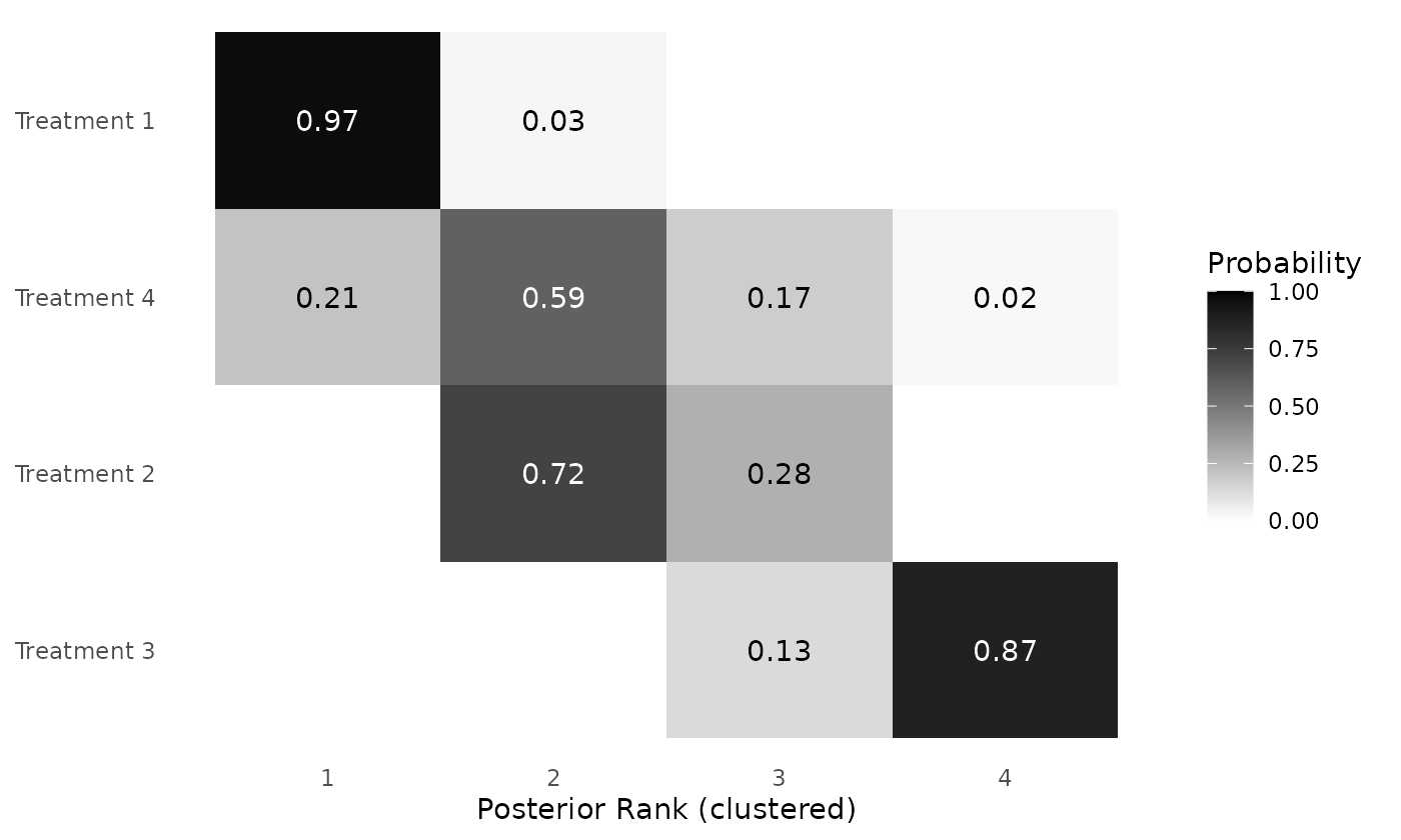
Figure 4: Posterior rank probabilities for each intervention in a toy example dataset, based on the RaCE-NMA model. Ranks are displayed on the ordinal scale (1 = best). Interventions are grouped into rank clusters representing non-exclusive superiority sets; multiple interventions within the same cluster may share identical posterior ranks.
The model estimates a 0.97 probability that Treatment 1 is in first place. Simultaneously, the model estimates a 0.21 probability that Treatment 4 is in first place. Thus, there is some probability, based on the model, that Treatments 1 and 4 are simultaneously the “best” treatments. That being said, Treatment 4 has substantial uncertainty in its rank, which aligns with the high uncertainty in original relative treatment effect data. Treatment 2 has a 0.72 probability of being in second place and Treatment 4 has a 0.87 probability of being in fourth (last) place.
The second function creates a cumulative ranking probability curve for each treatment. In words, the plot displays the probability that each treatment is at least in a specific rank place. For example, we see that Treatment 4 has a 0.80 probability of being in first or second place.
cumulativeprobplot_ranks(mcmc=mcmc_results_toy)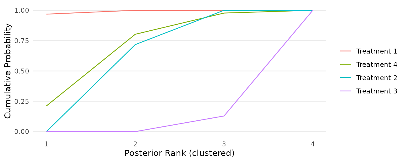
Figure 5: Cumulative ranking probability curves for each intervention in a toy example dataset, based on the RaCE-NMA model.
The third function creates a table displaying the SUCRA value and the
Median Number of Better Treatments (MNBT) for each treatment (with a
corresponding credible interval). The credible level may be specified
using the credible argument.
calculate_SUCRA_MNBT(mcmc=mcmc_results_toy, level = 0.5)
#>   Treatment      SUCRA MNBT (50% CI)
#> 1         1 0.98941667      0 (0, 0)
#> 2         4 0.66381667      1 (1, 1)
#> 3         2 0.57240000      1 (1, 2)
#> 4         3 0.04293333      3 (3, 3)
Real Data (Wang et. al [2022])
Next, we demonstrate the package on a real NMA study provided by Wang
et. al (2022) and analyzed as a Case Study in our paper. The data is
included in the RaCE.NMA package and can be loaded using
the following code:
data("wang_posterior")
round(head(wang_posterior), 3)
#>   R-CHOP-R R-Benda R-Benda-R R-Benda-R4 R-CVP R-CVP-R R-2(Len) G-CVP-G G-CHOP-G
#> 1   -0.471  -0.378    -0.986     -1.619 0.321   0.126   -0.314  -0.107   -0.698
#> 2   -0.425  -0.427    -1.060     -1.454 0.224   0.019   -0.390  -0.166   -0.572
#> 3   -0.378  -0.469    -0.987     -1.267 0.378   0.240   -0.245   0.123   -0.415
#> 4   -0.514  -0.404    -1.006     -1.423 0.216  -0.020   -0.568   0.192   -0.686
#> 5   -0.487  -0.289    -0.823     -1.017 0.223  -0.058   -0.419  -0.251   -0.610
#> 6   -0.322  -0.365    -0.769     -1.227 0.282   0.276   -0.283   0.084   -0.581
#>   G-Benda-G
#> 1    -1.294
#> 2    -1.433
#> 3    -1.242
#> 4    -1.288
#> 5    -1.157
#> 6    -1.091
It is important to note that wang_posterior only
includes relative treatment effects for non-baseline treatments. An 11th
treatment, “R-CHOP”, was the baseline with a relative treatment effect
of 0 by construction. Thus, for technical reasons described in the
paper, we will need to define summary statistics that can be used when
fitting the RaCE-NMA model.
# define assumed mean and variance for baseline treatment (R-CHOP)
mu_hat_baseline <- 0
var_baseline <- min(apply(wang_posterior,2,var))/10

# calculate summary statistics, mu_hat and cov
mu_hat_wang <- c( mu_hat_baseline, apply(wang_posterior,2,mean) )
cov_wang <- cbind( c(var_baseline, rep(0, 10) ),
              rbind(0, cov(wang_posterior)) )

# store treatment names
treatments <- c("R-CHOP", names(wang_posterior))
The following forest plot displays the relative treatment effects of the 11 treatments in the study, as estimated by Wang et. al (2022).
forestplot_muhat(data = cbind(0,wang_posterior),
                 names = treatments)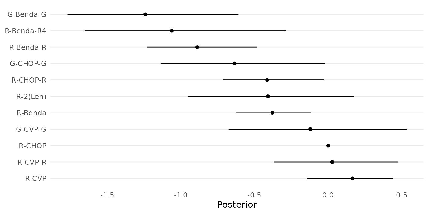
Figure 6: Forest plot of estimated relative treatment effects in a network meta-analysis by Wang et. al (2022), based on a standard NMA model.
Now, we proceed through the analysis pipeline.
1. Model Estimation
We fit the model below using 2 chains, each with MCMC iterations.
mcmc_results_casestudy <- mcmc_raceNMA(
  mu_hat = mu_hat_wang, cov = cov_wang,
  iter = 10000, nu_iter = 2, chains = 2, seed = 1
)
#> [1] "Estimating chain 1 of 2."
#> [1] "Estimating chain 2 of 2."
2. Model Assessment
Next, we view trace plots and convergence diagnostics.
traceplot_mu(mcmc_results_casestudy, names=treatments)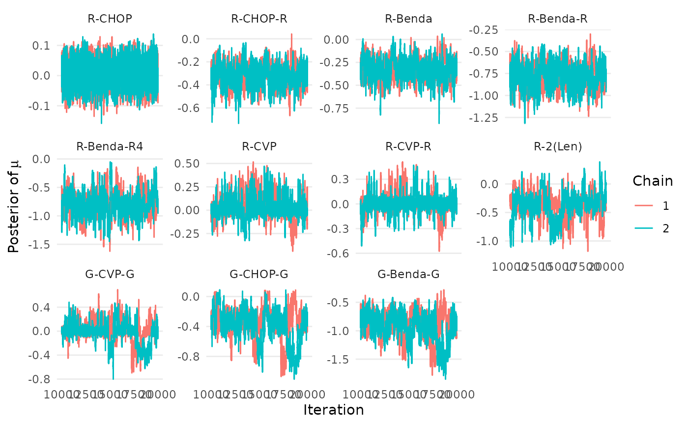
Figure 7: Trace plots of relative treatment effects in a network meta-analysis by Wang et. al (2022), based on the RaCE-NMA model.
traceplot_K(mcmc_results_casestudy)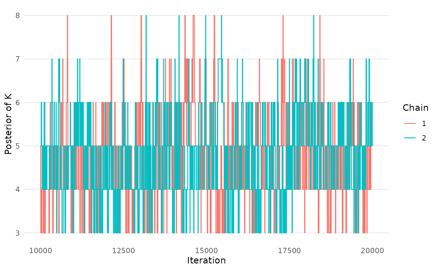
Figure 8: Trace plot of the number of rank-clusters, K, in a network meta-analysis by Wang et. al (2022), based on the RaCE-NMA model.
calculate_Rhat(mcmc_results_casestudy, names=treatments)
#> Potential scale reduction factors:
#>
#>            Point est. Upper C.I.
#> R-CHOP           1.00       1.01
#> R-CHOP-R         1.01       1.06
#> R-Benda          1.02       1.09
#> R-Benda-R        1.00       1.02
#> R-Benda-R4       1.00       1.00
#> R-CVP            1.08       1.30
#> R-CVP-R          1.09       1.32
#> R-2(Len)         1.16       1.55
#> G-CVP-G          1.08       1.31
#> G-CHOP-G         1.19       1.65
#> G-Benda-G        1.16       1.55
We observe that chains have not run long enough (refer to the Reproducibility tab for a longer run of chains). However, for demonstration purposes we continue with the next stage of the analysis pipeline below.
3. Inference and summary statistics
Disclaimer: The results below are based on chains which have not converged, but are shown for demonstration purposes. Please see the Reproducibility tab for accurate results based on this data.
clusterplot_ranks(mcmc=mcmc_results_casestudy, names = treatments, label_ranks = 1)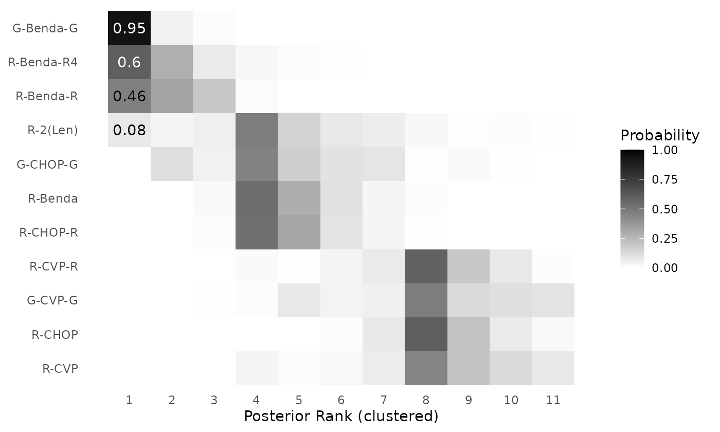
Figure 9: Posterior rank probabilities for each intervention in a network meta-analysis by Wang et. al (2022), based on the RaCE-NMA model. Ranks are displayed on the ordinal scale (1 = best). Interventions are grouped into rank clusters representing non-exclusive superiority sets; multiple interventions within the same cluster may share identical posterior ranks.
cumulativeprobplot_ranks(mcmc=mcmc_results_casestudy, names=treatments)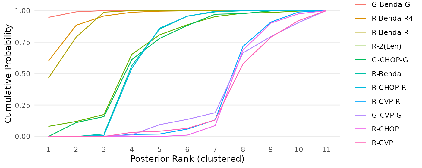
Figure 10: Cumulative ranking probability curves for each intervention in a network meta-analysis by Wang et. al (2022), based on the RaCE-NMA model.
calculate_SUCRA_MNBT(mcmc=mcmc_results_casestudy,names=treatments,level=0.50)
#>     Treatment    SUCRA MNBT (50% CI)
#> 1   G-Benda-G 0.993630      0 (0, 0)
#> 2  R-Benda-R4 0.942055      0 (0, 1)
#> 3   R-Benda-R 0.924070      1 (0, 1)
#> 4    R-2(Len) 0.663695      3 (3, 4)
#> 5    G-CHOP-G 0.648690      3 (3, 4)
#> 6     R-Benda 0.637975      3 (3, 4)
#> 7    R-CHOP-R 0.636165      3 (3, 4)
#> 8     R-CVP-R 0.284175      7 (7, 8)
#> 9     G-CVP-G 0.279990      7 (7, 8)
#> 10     R-CHOP 0.266110      7 (7, 8)
#> 11      R-CVP 0.255875      7 (7, 8)