class: center, top, title-slide .title[ # CSSS 508, Lecture 3 ] .subtitle[ ## Manipulating and Summarizing Data ] .author[ ### Michael Pearce<br>(based on slides from Chuck Lanfear) ] .date[ ### April 12, 2022 ] --- class: inverse # Topics Last time, we learned about, 1. Useful coding tips: packages, directories, and saving data 1. Basics of ggplot: layers and aesthetics 1. Advanced ggplot tools -- Today, we will cover, 1. Building blocks 1. Subsetting data 1. Modifying data 1. Summarizing data 1. Merging together data --- class: inverse # Death to Spreadsheets Tools like *Excel* or *Google Sheets* lets you manipulate spreadsheets using functions. * Spreads are *not reproducible*: It's hard to know how someone changed the raw data! * It's hard to catch mistakes when you use spreadsheets. Don't be the next sad Research Assistant who makes headlines with an Excel error! ([Reinhart & Rogoff, 2010](http://www.bloomberg.com/news/articles/2013-04-18/faq-reinhart-rogoff-and-the-excel-error-that-changed-history)) Today, we'll use R to manipulate data more *transparently* and *reproducibly*. --- class:inverse # 1. Building Blocks 1. Logical Operators (`!=`, `==`, `>`, `<=`, etc. ) 1. Combining Logical Operators (`&`, `|`) --- ## Logical Operators Logical operators refer to base functions which allow us to **test a connection** between two objects. -- For example, we may test + Is A equal to B? + Is A greater than B? + Is A within B? and many others! --- ## Logical Operators in Code * `==`: is equal to (note: there are TWO equal signs here!) -- * `!=`: not equal to -- * `>`, `>=`, `<`, `<=`: less than, less than or equal to, etc. -- * `%in%`: used with checking equal to one of several values --- ## Examples of Logical Operators Let's create two objects, `A` and `B` ```r A <- c(5,10,15) B <- c(5,15,25) ``` -- ```r A == B ``` ``` ## [1] TRUE FALSE FALSE ``` ```r A > B ``` ``` ## [1] FALSE FALSE FALSE ``` ```r A %in% B ``` ``` ## [1] TRUE FALSE TRUE ``` --- ## Combining Logical Operators We have three main ways to combine logical operators: * `&`: **both** conditions need to hold (AND) -- * `|`: **at least one** condition needs to hold (OR) -- * `!`: **inverts** a logical condition (`TRUE` becomes `FALSE`, `FALSE` becomes `TRUE`) --- ## Examples ```r A <- c(5,10,15); B <- c(5,15,25) ``` -- ```r A > 5 & A <= B ``` ``` ## [1] FALSE TRUE TRUE ``` ```r B < 10 | B > 20 ``` ``` ## [1] TRUE FALSE TRUE ``` ```r !(A == 10) ``` ``` ## [1] TRUE FALSE TRUE ``` --- class: inverse # Aside: `dplyr` Today, we'll use tools from the `dplyr` package to manipulate data! + Like `ggplot2`, `dplyr` is part of the *Tidyverse*, a modern collection of data science tools introduced by Hadley Wickham. + You can read more about the tidyverse on its [website](http://tidyverse.org/). -- To get started, let's install (in the console) and load (in an R/Rmd file) dplyr. (We also load `gapminder`!) ```r # install.packages("dplyr") library(dplyr) library(gapminder) ``` --- ## Building Block of `dplyr`: Pipes `dplyr` allows us to use the "pipe" data between functions using the (`%>%`) operator. So instead of nesting functions like this: ```r log(mean(gapminder$pop)) ``` ``` ## [1] 17.20333 ``` -- We can **pipe** them like this: ```r gapminder$pop %>% mean() %>% log() ``` ``` ## [1] 17.20333 ``` -- + Pipes read "left to right" (intuitive) + Nested functions read "inside to out." (kinda weird) --- class: inverse # 2. Subsetting data + `filter()` + `select()` + `distinct()` --- ## Subset Rows: `filter` We often get *big* datasets, and we only want some of the entries. We can subset rows using `filter`. -- ```r gapminder %>% filter(country == "China") %>% head(4) # display first four rows ``` ``` ## # A tibble: 4 × 6 ## country continent year lifeExp pop gdpPercap ## <fct> <fct> <int> <dbl> <int> <dbl> ## 1 China Asia 1952 44 556263527 400. ## 2 China Asia 1957 50.5 637408000 576. ## 3 China Asia 1962 44.5 665770000 488. ## 4 China Asia 1967 58.4 754550000 613. ``` ```r China <- gapminder %>% filter(country == "China") ``` (Now, `China` is an object in our environment which contains rows corresponding to China.) --- ## Subset Columns: `select` What if we want to keep each entry, but only use certain variables? Use `select`! -- ```r gapminder %>% select(country,continent,year,lifeExp) %>% head(4) ``` ``` ## # A tibble: 4 × 4 ## country continent year lifeExp ## <fct> <fct> <int> <dbl> ## 1 Afghanistan Asia 1952 28.8 ## 2 Afghanistan Asia 1957 30.3 ## 3 Afghanistan Asia 1962 32.0 ## 4 Afghanistan Asia 1967 34.0 ``` --- ## Dropping columns with `select` Alternatively, we can use `select()` to drop variables using a `-` sign: ```r gapminder %>% select(-continent, -pop, -lifeExp) %>% head(4) ``` ``` ## # A tibble: 4 × 3 ## country year gdpPercap ## <fct> <int> <dbl> ## 1 Afghanistan 1952 779. ## 2 Afghanistan 1957 821. ## 3 Afghanistan 1962 853. ## 4 Afghanistan 1967 836. ``` --- ## Finding Unique Rows: `distinct` You may want to find the unique combinations of variables in a dataset. Use `distinct` -- ```r gapminder %>% distinct(continent, year) %>% head(6) ``` ``` ## # A tibble: 6 × 2 ## continent year ## <fct> <int> ## 1 Asia 1952 ## 2 Asia 1957 ## 3 Asia 1962 ## 4 Asia 1967 ## 5 Asia 1972 ## 6 Asia 1977 ``` --- ## `distinct` drops variables! By default, `distinct()` drops unused variables. If you don't want to drop them, add the argument `.keep_all=TRUE`: ```r gapminder %>% distinct(continent, year, .keep_all=TRUE) %>% head(6) ``` ``` ## # A tibble: 6 × 6 ## country continent year lifeExp pop gdpPercap ## <fct> <fct> <int> <dbl> <int> <dbl> ## 1 Afghanistan Asia 1952 28.8 8425333 779. ## 2 Afghanistan Asia 1957 30.3 9240934 821. ## 3 Afghanistan Asia 1962 32.0 10267083 853. ## 4 Afghanistan Asia 1967 34.0 11537966 836. ## 5 Afghanistan Asia 1972 36.1 13079460 740. ## 6 Afghanistan Asia 1977 38.4 14880372 786. ``` --- class: inverse # 3. Modifying data + `arrange()` + `rename()` + `mutate()` --- ## Sorting data by rows: `arrange` Sometimes it's useful to sort rows in your data, in ascending (low to high) or descending (high to low) order. We do that with `arrange`. -- ```r US_and_Canada <- gapminder %>% filter(country %in% c("United States","Canada")) US_and_Canada %>% arrange(year,lifeExp) %>% head(4) ``` ``` ## # A tibble: 4 × 6 ## country continent year lifeExp pop gdpPercap ## <fct> <fct> <int> <dbl> <int> <dbl> ## 1 United States Americas 1952 68.4 157553000 13990. ## 2 Canada Americas 1952 68.8 14785584 11367. ## 3 United States Americas 1957 69.5 171984000 14847. ## 4 Canada Americas 1957 70.0 17010154 12490. ``` --- ## Sorting data by rows: `arrange` To sort in descending order, using `desc()` within `arrange` ```r US_and_Canada %>% arrange(desc(pop)) %>% head(4) ``` ``` ## # A tibble: 4 × 6 ## country continent year lifeExp pop gdpPercap ## <fct> <fct> <int> <dbl> <int> <dbl> ## 1 United States Americas 2007 78.2 301139947 42952. ## 2 United States Americas 2002 77.3 287675526 39097. ## 3 United States Americas 1997 76.8 272911760 35767. ## 4 United States Americas 1992 76.1 256894189 32004. ``` --- ## Rename variables: `rename` You may receive data with unintuitive variable names. You can change them using `rename()`. -- ```r US_and_Canada %>% rename(life_expectancy = lifeExp) %>% head(4) ``` ``` ## # A tibble: 4 × 6 ## country continent year life_expectancy pop gdpPercap ## <fct> <fct> <int> <dbl> <int> <dbl> ## 1 Canada Americas 1952 68.8 14785584 11367. ## 2 Canada Americas 1957 70.0 17010154 12490. ## 3 Canada Americas 1962 71.3 18985849 13462. ## 4 Canada Americas 1967 72.1 20819767 16077. ``` -- (NOTE 1: I did *not* re-save the object `US_and_Canada`, so the name change is *not* permanent!) (NOTE 2: I recommend **against** using spaces in a name! It makes things *really hard* sometimes!!) --- ## Create new columns: `mutate` You can add new columns to a data frame using `mutate()`. -- For example, perhaps we wish to state the population in millions: ```r US_and_Canada %>% select(country, year, pop) %>% * mutate(pop_millions = pop / 1000000) %>% head(5) ``` ``` ## # A tibble: 5 × 4 ## country year pop pop_millions ## <fct> <int> <int> <dbl> ## 1 Canada 1952 14785584 14.8 ## 2 Canada 1957 17010154 17.0 ## 3 Canada 1962 18985849 19.0 ## 4 Canada 1967 20819767 20.8 ## 5 Canada 1972 22284500 22.3 ``` --- class: inverse # 4. Summarizing data + `summarize()` + `group_by()` --- ## Summarizing data: `summarize` **`summarize()`** calculates summaries of variables in your data: * Count the number of rows * Calculate the mean * Calculate the sum * Find the minimum or maximum value You can use any function inside `summarize()` that aggregates *multiple values* into a *single value* (like `sd()`, `mean()`, or `max()`). --- ## `summarize()` Example For the year 1982, let's summarize some values in `gapminder` ```r gapminder %>% filter(year == 1982) %>% summarize(number_observations = n(), max_lifeexp = max(lifeExp), mean_pop = mean(pop), sd_pop = sd(pop)) ``` ``` ## # A tibble: 1 × 4 ## number_observations max_lifeexp mean_pop sd_pop ## <int> <dbl> <dbl> <dbl> ## 1 142 77.1 30207302. 105098650. ``` --- ## Summarizing data by groups: `group_by` What if we want to summarize data by category? Use `group_by` **and** `summarize` -- Functions after `group_by()` are computed *within each group* as defined by variables given, rather than over all rows at once. --- ## `group_by()` Example ```r *US_and_Canada %>% group_by(year) %>% * summarize(total_pop = sum(pop)) %>% head(4) ``` ``` ## # A tibble: 4 × 2 ## year total_pop ## <int> <int> ## 1 1952 172338584 ## 2 1957 188994154 ## 3 1962 205523849 ## 4 1967 219531767 ``` Because we did `group_by()` with `year` then used `summarize()`, we get *one row per value of `year`*! --- class:inverse # 5. Merging together data + `left_join()` + `full_join()` --- ## Why merge?! In practice, we often collect data from different sources. To analyze the data, we usually must first combine (merge) them. -- For example, imagine you would like to study county-level patterns with respect to age and grocery spending. However, you can only find, * County level age data from the US Census, and * County level grocery spending data from the US Department of Agriculture -- Merge the data!! --- ## Merging in Concept When merging datasets `A` and `B`, ask yourself the following two questions: -- * Which **rows** do I want to keep? + All rows in `A`? + All rows in both `A` and `B`? -- * How do my datasets **connect**? + Is there a specific variable they have in common? + Multiple variables they have in common? --- ## Which Rows to Keep: We'll focus on two types of joins:<sup>1</sup>... * `A %>% left_join(B)`: keeps `A` and adds variables from `B` after matching. * `A %>% full_join(B)`: keeps all of `A` and `B`, but combines rows when possible. .footnote[[1] Other types include `right_join`, `inner_join`, `semi_join`, and `anti_join`, but we won't study those here.] --- ## Matching Criteria We have to tell R **which variables** to use when merging datasets! Rows are matched when the values in matching variables are equivalent. -- * `by = c("County")`: Both datasets have a `County` variable, match on this! -- * `by = c("CountyName" = "County_Name")`: Match `CountyName` in `A` with `County_Name` in `B` --- ## Example: `nycflights13` Data The `nycflights13` package includes five data frames, some of which contain missing data (`NA`): * `flights`: flights leaving JFK, LGA, or EWR in 2013 * `airlines`: airline abbreviations * `airports`: airport metadata * `planes`: airplane metadata * `weather`: hourly weather data for JFK, LGA, and EWR .smallish[ ```r # install.packages("nycflights13") library(nycflights13) ``` ] --- ## Join Example 1 `flights` has one row per flight, with abbreviated airline names. ```r flights %>% select(flight,origin,dest,carrier) %>% head(2) ``` ``` ## # A tibble: 2 × 4 ## flight origin dest carrier ## <int> <chr> <chr> <chr> ## 1 1545 EWR IAH UA ## 2 1714 LGA IAH UA ``` -- `airlines` has one row per airline, with airline abbreviations *and* full names ```r airlines %>% head(2) ``` ``` ## # A tibble: 2 × 2 ## carrier name ## <chr> <chr> ## 1 9E Endeavor Air Inc. ## 2 AA American Airlines Inc. ``` --- ## Join Example 1 (continued) Let's left join `flights` with `airlines` to add full airline name to each flight record! ```r flights %>% select(flight,origin,dest,carrier) %>% * left_join(airlines, by = "carrier") %>% head(5) ``` ``` ## # A tibble: 5 × 5 ## flight origin dest carrier name ## <int> <chr> <chr> <chr> <chr> ## 1 1545 EWR IAH UA United Air Lines Inc. ## 2 1714 LGA IAH UA United Air Lines Inc. ## 3 1141 JFK MIA AA American Airlines Inc. ## 4 725 JFK BQN B6 JetBlue Airways ## 5 461 LGA ATL DL Delta Air Lines Inc. ``` We now have one row per flight, with both carrier abbreviations and full names! --- ## Join Example #2 `flights` also includes a `tailnum` variable for each plane's tail number. ```r flights %>% select(flight,origin,dest,tailnum) %>% head(2) ``` ``` ## # A tibble: 2 × 4 ## flight origin dest tailnum ## <int> <chr> <chr> <chr> ## 1 1545 EWR IAH N14228 ## 2 1714 LGA IAH N24211 ``` -- `planes` includes a row for each plane type, including the manufacturer. ```r planes %>% select(tailnum,year,manufacturer,model) %>% head(2) ``` ``` ## # A tibble: 2 × 4 ## tailnum year manufacturer model ## <chr> <int> <chr> <chr> ## 1 N10156 2004 EMBRAER EMB-145XR ## 2 N102UW 1998 AIRBUS INDUSTRIE A320-214 ``` --- ## Join Example 2 (continued) Let's left join `flights` with `planes` to add manufacture to each flight record! ```r flights %>% select(flight,origin,dest,tailnum) %>% * left_join(planes, by = "tailnum") %>% head(5) ``` ``` ## # A tibble: 5 × 12 ## flight origin dest tailnum year type manuf…¹ model engines seats speed engine ## <int> <chr> <chr> <chr> <int> <chr> <chr> <chr> <int> <int> <int> <chr> ## 1 1545 EWR IAH N14228 1999 Fixed wing m… BOEING 737-… 2 149 NA Turbo… ## 2 1714 LGA IAH N24211 1998 Fixed wing m… BOEING 737-… 2 149 NA Turbo… ## 3 1141 JFK MIA N619AA 1990 Fixed wing m… BOEING 757-… 2 178 NA Turbo… ## 4 725 JFK BQN N804JB 2012 Fixed wing m… AIRBUS A320… 2 200 NA Turbo… ## 5 461 LGA ATL N668DN 1991 Fixed wing m… BOEING 757-… 2 178 NA Turbo… ## # … with abbreviated variable name ¹manufacturer ``` A bunch of columns from `planes` are now in the dataset! --- ## Join Example 2 (continued) Let's remove some of the "spare" columns ```r flights %>% select(flight,origin,dest,tailnum) %>% left_join(planes, by = "tailnum") %>% * select(flight,origin,dest,manufacturer,model) %>% head(5) ``` ``` ## # A tibble: 5 × 5 ## flight origin dest manufacturer model ## <int> <chr> <chr> <chr> <chr> ## 1 1545 EWR IAH BOEING 737-824 ## 2 1714 LGA IAH BOEING 737-824 ## 3 1141 JFK MIA BOEING 757-223 ## 4 725 JFK BQN AIRBUS A320-232 ## 5 461 LGA ATL BOEING 757-232 ``` --- class: inverse # Summary 1. Logical Operators (`&, |, ==, <, %in%,` etc.) 1. Subsetting (`filter, select, distinct`) 1. Modifying (`arrange, rename, mutate`) 1. Summarizing (`summarize, group_by`) 1. Merging (`left_join, full_join`) Let's take a 10-minute break, then come back together to practice! --- class:inverse # Activity 1. Create a new object that contains `gapminder` (1) observations from China, India, and United States after 1980, and (2) variables corresponding to country, year, population, and life expectancy. 1. How many rows and columns does the object contain? 1. Save over your object after sorting the rows by year (ascending order) and population (descending order). Print the first 6 rows. 1. Add a new variable that contains population in billions. 1. By year, calculate the total population (in billions) across these three countries 1. In ggplot, create a line plot showing life expectancy over time by country. Make the plot visually appealing! --- # My Answers Question 1: ```r subset_gapminder <- gapminder %>% filter(country %in% c("China","India","United States"), year >1980 ) %>% select(country, year, pop, lifeExp) ``` -- Question 2: ```r c(nrow(subset_gapminder),ncol(subset_gapminder)) ``` ``` ## [1] 18 4 ``` --- # My Answers Question 3: ```r subset_gapminder <- subset_gapminder %>% arrange(year,desc(pop)) subset_gapminder %>% head(6) ``` ``` ## # A tibble: 6 × 4 ## country year pop lifeExp ## <fct> <int> <int> <dbl> ## 1 China 1982 1000281000 65.5 ## 2 India 1982 708000000 56.6 ## 3 United States 1982 232187835 74.6 ## 4 China 1987 1084035000 67.3 ## 5 India 1987 788000000 58.6 ## 6 United States 1987 242803533 75.0 ``` -- Question 4: ```r subset_gapminder <- subset_gapminder %>% mutate(pop_billions = pop/1000000000) ``` --- # My Answers Question 5: ```r subset_gapminder %>% group_by(year) %>% summarize(TotalPop_Billions = sum(pop_billions)) ``` ``` ## # A tibble: 6 × 2 ## year TotalPop_Billions ## <int> <dbl> ## 1 1982 1.94 ## 2 1987 2.11 ## 3 1992 2.29 ## 4 1997 2.46 ## 5 2002 2.60 ## 6 2007 2.73 ``` --- # My Answers .small[ Question 6 ```r library(ggplot2) ggplot(subset_gapminder,aes(year,lifeExp,color=country,group=country))+ theme_bw(base_size=20)+geom_point()+geom_line()+ xlab("Year")+ylab("Life Expectancy (years)")+ ggtitle("Life Expectancy (1982-2007)","China, India, and United States")+ scale_x_continuous(breaks=c(1982,1987,1992,1997,2002,2007),minor_breaks = c())+ ylim(c(50,80))+scale_color_discrete(name="Country")+theme(legend.position = "bottom") ``` 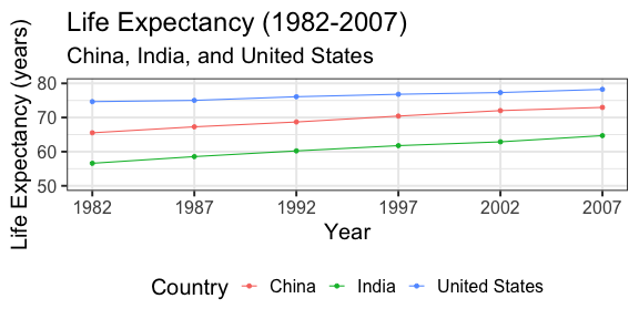<!-- --> ] --- # Homework 3 .small[ Create an RMarkdown file (from scratch this time!) in which you answer each of the following questions. Be sure to display **all your code in the knitted** version (use throughout `echo=TRUE`). Remember, the package `nycflights13` contains data on flights originating in NYC during the year 2013. There are three airports servicing NYC: JFK, LGA ("LaGuardia"), and EWR ("Newark"). 1. Choose an airport outside New York, and count how many flights went to that airport from NYC in 2013. How many of those flights started at JFK, LGA, and EWR? (Hint: Use `filter`, `group_by`, and `summarize`) 1. The variable `arr_delay` contains arrival delays in minutes (negative values represent early arrivals). Make a `ggplot` histogram displaying arrival delays for 2013 flights from NYC to the airport you chose. 1. Use `left_join` to add weather data at departure to the subsetted data (Hint 1: Match on `origin`, `year`, `month`, `day`, **and** `hour`!!). Calculate the mean temperature by month at departure (`temp`) across all flights (Hint 2: Use `mean(temp,na.rm=T)` to have R calculate an average after ignoring missing data values). 1. Investigate if there is a relationship between departure delay (`dep_delay`) and wind speed (`wind_speed`). Is the relationship different between JFK, LGA, and EWR? I suggest answering this question by making a plot and writing down a one-sentence interpretation. As always, submit both the .Rmd and knitted .html to Canvas. ]